Inverse Kinematic - An Introduction with Robotics & CPS Examples - Forward vs Inverse Kinematics

If you’ve ever watched a robot arm pick up a part, a drone gimbal stabilize a camera, or a humanoid place its foot precisely on the ground, you’ve seen kinematics in action. Kinematics is the branch of mechanics that describes motion without talking about forces.

The theory behind kinematics involves the calculation of joint and end-effector positions. It answers questions like:

“If I rotate these joints by these angles, where does the end-effector end up?”
“If I want the end-effector to be here, what joint angles should I command?”

Inverse kinematics is the use of kinematic equations to determine the motion of a robot to reach a desired position.

Those two questions define the classic pair:

Forward Kinematics (FK): joint values → pose (position + orientation)
Inverse Kinematics (IK): desired pose → joint values. This involves the calculation of joint values to achieve a desired pose, and these values are often calculated using analytical or numerical methods.

This article is a step-by-step, beginner-friendly introduction to FK vs IK, with concrete robotics, physical AI and cyber-physical systems (CPS) examples, plus practical intuition about why IK is harder and how it’s typically solved.

1) Frames, Poses, and Why Robots Need Math

Robots live in the physical world, but their controllers live in a world of numbers. To command a robot, we need a mapping between:

Joint space: the variables you can directly control or measure
e.g., joint angles (revolute joints), joint displacements (prismatic joints)
Joint positions: the specific values assigned to each joint that define the robot’s configuration
Task space (Cartesian space): what you actually care about
e.g., end-effector position (x, y, z) and orientation (roll, pitch, yaw)

To connect these, we define reference frames:

A base frame attached to the robot’s base (or world)
A tool frame attached to the end-effector (gripper, camera, welding torch)
The robot model defines how these frames are attached to the robot’s structure, including the assignment of coordinate axes.

When describing the base and tool frames in robot kinematics, the z axis is typically assigned along the axis of motion for each joint (e.g., the axis of rotation for revolute joints), while the x axis is chosen according to the Denavit-Hartenberg convention to ensure consistent orientation and facilitate kinematic calculations.

A pose is typically represented as:

Position: p = (x, y, z)
Orientation: a rotation matrix R, or quaternion, or Euler angles
Combined as a homogeneous transform:

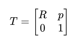
T=[R0p1]

This “T” is the standard way to move between coordinate frames.

2) What Forward Kinematics Means (FK)

The FK question

“Given my joint values, where is the end-effector?”

So FK is a function:

pose=f(joints)

Forward kinematics uses kinematic equations to map joint values to the end-effector pose.

Why FK is usually “easy”

For most manipulators, FK is computed by chaining transforms from one link to the next. If you know:

link lengths
joint axes
joint values

…you can compute the end-effector pose deterministically.

A simple 2D example: a 2-link planar arm

Imagine a robotic arm moving in a plane with:

link lengths: L1, L2
joint angles: θ1, θ2

Diagram (top view):

1
2
3

Base o----(L1)----o----(L2)----X  End-effector
       θ1      θ2 (relative to link1)

The end-effector position is:

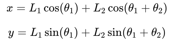
x=L1cos(θ1)+L2cos(θ1+θ2)
y=L1sin(θ1)+L2sin(θ1+θ2)

That’s forward kinematics: plug in angles → get (x, y).

FK in real CPS terms

Forward kinematics is what your system uses when:

encoders measure joint angles,
you calculate where the tool actually is,
you then compare to a target (for feedback, monitoring, safety, logging, etc.).

Examples:

Robot arm: the current gripper pose is calculated from encoder readings.
Gimbal: compute camera orientation from motor angles.
Legged robot: compute foot position from hip/knee/ankle joint angles.

3) What Inverse Kinematics Means (IK)

The IK question

“Given the pose I want, what joint values produce it?”

In inverse kinematic (IK), the joint values are calculated to achieve the desired pose.

So IK is the “inverse” function:

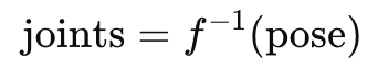
joints=f−1(pose)

Why IK is “harder”

IK is harder than FK because it can be:

Non-unique (multiple solutions)
A robot arm can often reach the same point with different elbow configurations.
Sometimes impossible (no solution)
Target is outside the robot’s reachable workspace, or violates joint limits.
Numerically tricky (singularities / instability)
Certain configurations make small Cartesian changes require huge joint changes.
Constrained
Real robots have:

joint limits
collision constraints
preferred postures
velocity/acceleration limits
task-specific constraints (keep tool vertical, avoid cables, etc.)

Same 2-link planar arm: multiple IK solutions

For a point (x, y) within reach, the arm often has two configurations, each resulting in a different final pose for the robotic arm:

Elbow-up:     Elbow-down:
   o              o
  / \            / \
 o   X          o   X

So IK must decide which final pose you want (or pick one based on a rule).

4) Workspace, Reachability, and Constraints

Before solving IK, you should know the workspace:

The set of all end-effector positions/orientations the robot can reach.
The initial position of the robot arm is important, as it determines the starting point for motion planning and affects the motion profile needed to reach the target.

For the 2-link planar arm:

Maximum reach: L1 + L2
Minimum reach (if it can fold back): |L1 - L2|

So a target is reachable only if:

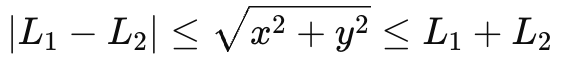
∣L1−L2∣ ≤ x2+y2 ≤ L1+L2

In real CPS, IK is almost never “just math”; it’s math + constraints:

“Reach the point, but don’t collide with the table.”
“Avoid collisions with an object in the workspace.”
“Keep the camera pointing at the target.”
“Don’t exceed joint 4’s limit.”
“Avoid near-singular postures.”

5) End Effectors: The Robot’s “Hand” in the World

End effectors are the “hands” of robots, the components at the tip of a robot arm that actually interact with the physical environment. Whether it’s a gripper picking up a part, a welding torch joining metal, or a suction cup moving glass, the end effector is what allows a robot to perform useful work in the real world. In the context of cyber physical systems, end effectors are the crucial link between intelligent control algorithms and the physical processes they automate.

The end effector sits at the end of the robot’s kinematic chain, and its position and orientation (pose) are the ultimate goal of most robot motion. To achieve a desired position or orientation for the end effector, control systems use kinematics equations—forward kinematics to determine where the end effector is given the current joint angles, and inverse kinematics to calculate the joint parameters needed to reach a target pose. This mapping is essential for precise automation, especially in environments where robots must interact with humans or other devices.

Designing an end effector involves more than just mechanical engineering. Human interaction is a key consideration, especially for collaborative robots (cobots) that share workspaces with people. Factors like ergonomics, safety, and efficiency must be balanced, ensuring that the end effector can perform its tasks without risking harm to humans or damaging objects. For example, a collaborative robot in manufacturing might use a soft gripper with force sensors to safely handle delicate parts alongside human workers.

Control algorithms and software components play a vital role in managing end effector motion. These systems translate high-level commands, such as a desired end effector position or orientation, into low-level joint movements, using real-time data and historical data to optimize performance. In process control and civil infrastructure applications, end effectors might be used to manipulate valves, assemble components, or even perform maintenance tasks in hazardous environments, all under the watchful eye of intelligent control systems.

Modern end effectors often integrate advanced technologies like artificial intelligence and computer vision, enabling them to adapt to changing environments and perform complex tasks. For instance, a robot equipped with a vision-guided end effector can identify and grasp objects of varying shapes and sizes, adjusting its grip in real time based on sensor feedback. The Jacobian matrix is a key mathematical tool in this process, relating changes in joint angles to changes in the end effector’s position and orientation along the x, y, and z axes.

Degrees of freedom are another critical aspect of end effector design. The more degrees of freedom an end effector has, the greater its flexibility and range of motion—allowing it to reach around obstacles, orient tools precisely, or perform intricate assembly tasks. Other data, such as force and torque measurements, are also essential for tasks that require delicate manipulation or feedback-based control.

Robotics research continues to push the boundaries of what end effectors can do, using both numerical solutions and analytic solutions to optimize their design and control. The CPS program and advances in cps technologies have accelerated the integration of end effectors into a wide range of applications, from manufacturing and automation to civil infrastructure and beyond.

In summary, end effectors are the business end of robots, enabling them to interact with and manipulate their environment. Their design and control are deeply intertwined with kinematics, control algorithms, and the broader goals of cyber physical systems. As robots become more capable and collaborative, the importance of intelligent, safe, and efficient end effectors will only continue to grow.

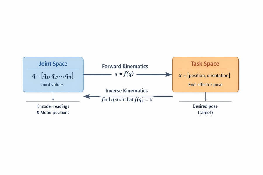
5) A Practical Mental Model: Two Spaces and a Mapping

A helpful way to think about it:

There are two spaces: joint space and task space. Joint space is defined by the variables that control each joint of the robot, such as angles or displacements. The specific values assigned to each joint variable are called joint positions. Task space, on the other hand, describes the position and orientation of the robot’s end effector in the environment. Mapping between these spaces is the core of kinematics.

Joint space (what motors understand)

A vector:

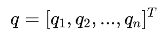
q=[q1,q2,...,qn]T

Task space (what humans specify)

A pose:

x=[p,  orientation]

FK is a direct mapping

x=f(q)

IK is “find q such that f(q) = x”

That’s a search problem, not just a formula—especially for complex robots.

6) How IK is Actually Solved in Practice

There are two big families of IK methods: analytic solutions and numerical approaches. Inverse kinematic problems can be solved using either an analytic solution, which provides a closed-form answer, or a numerical approach, which relies on iterative calculation to determine the joint configurations needed for the robot to reach a desired position.

Analytical IK

Analytical solutions are possible when the kinematic equations can be solved exactly. Analytical inverse kinematic solutions are best suited for robots with low degrees of freedom due to the nonlinearity of the kinematics equations.

Numerical IK

Numerical methods use iterative calculation to approximate the joint angles that achieve the target end-effector position. Numerical inverse kinematic solutions require multiple steps to converge toward the solution due to the non-linearity of the system.

A) Analytical (closed-form) IK

An analytic solution is an explicit, closed-form solution to the inverse kinematic (IK) problem, where you derive explicit equations and solve them symbolically.

Pros:

fast
exact (within math assumptions)
can enumerate multiple solutions

Cons:

not always possible to derive (especially for complex geometries)
harder to maintain and extend with constraints

Analytical inverse kinematic solutions are best suited for robots with low degrees of freedom due to the nonlinearity of the kinematics equations.

Many classic 6-DOF industrial arms are designed to make analytical IK possible.

B) Numerical (iterative) IK

You start from a guess and iteratively improve it.

High-level idea:

Start with a current joint estimate q0q
Compute the current end-effector pose x0=f(q0)
Compute the error e=xtarget−x0
Update joints a little to reduce error
Repeat until error is small enough or you hit a limit

A core tool here is the Jacobian.

7) The Jacobian: The Bridge Between Small Motions

The Jacobian J(q) relates joint velocities to end-effector velocities:

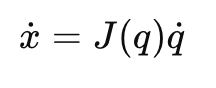
x˙=J(q)q˙

Interpretation:

If you move joints a tiny bit, how does the end-effector move?

For IK (position/orientation), we often use it like this:

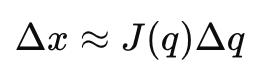
Δx≈J(q)Δq

So we can choose:

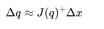
Δq≈J(q)+Δx

where J+J^{+}J+ is a pseudo-inverse (because J might not be square). The calculation of joint updates in inverse kinematic problems relies on the Jacobian matrix, especially when using numerical calculation methods to determine the required joint angles.

Why singularities matter

A singularity is a configuration where the robot loses the ability to move in some Cartesian direction (or requires infinite joint speed to do so). Numerically:

the Jacobian becomes ill-conditioned
small desired Cartesian steps produce huge joint steps

In CPS terms, singularities can show up as:

jittery joints
unstable commands
unexpected posture flips
inability to track a smooth tool path

8) A Concrete Robotics Example: “Move the Gripper Here”

Problem

You want a gripper to move to a point above a part on a conveyor.

Task space target: desired end effector pose, e.g., “position at (x, y, z), tool pointing down”
IK solver computes joint angles
Controller drives motors to those angles
FK is used to verify where the tool is during motion

Typical pipeline:

Desired end effector pose (task space)
        |
        v
   IK solver (constraints, limits, posture)
        |
        v
 Joint targets q*
        |
        v
 Motor controllers + sensors
        |
        v
 Encoder readings q(t)
        |
        v
 FK -> estimated end-effector pose x(t)
        |
        v
 Compare x(t) vs target, monitor errors, safety

This is the FK/IK pairing in the real world: IK plans, FK monitors.

9) A CPS Example Beyond Arms: A Camera Gimbal

A 3-axis gimbal is a cyber-physical system (physical AI) with:

motors (actuators)
IMU sensors
computational elements such as microprocessors and control algorithms
a control loop

If the system wants “camera points at heading 30°, pitch -10°”:

The system must focus on specific orientations or targets to achieve accurate camera alignment.
IK-like mapping: desired orientation → motor angles
FK-like mapping: motor angles → predicted camera orientation

In practice, many gimbals use orientation representations (quaternions/rotation matrices) and constraints like:

limit roll range
avoid cable wrap
smooth transitions (no sudden flips)

Even though it’s not an “arm”, it’s the same concept: actuator space ↔ task space.

10) Typical IK Pitfalls (and How Engineers Handle Them)

Pitfall 1: Multiple solutions

Symptom: arm suddenly “elbow flips” to another posture.

Common fixes:

choose the solution closest to the current joints (minimize |q - q_current|)
add a posture preference (“keep elbow up”)
add continuity constraints (avoid big jumps)

Pitfall 2: Unreachable targets

Symptom: solver diverges, or joints hit limits.

Common fixes:

project target into reachable workspace
return a “best effort” solution with minimal error
fail fast and re-plan

Pitfall 3: Joint limits and collisions

Symptom: mathematically valid IK is physically unsafe.

Common fixes:

constrained numerical solvers (optimization-based IK)
collision checking integrated into planning
add penalties for near-limit joints

Pitfall 4: Singularities

Symptom: near a straight-arm configuration, tiny motion → crazy joint motion.

Common fixes:

damped least squares (adds stability)
singularity avoidance terms
re-plan path to avoid problematic configurations

11) “Forward vs Inverse” in One Sentence Each

Forward kinematics: “Tell me where I am.”
FK is a straightforward calculation that determines the end-effector position from given joint angles.
Inverse kinematics: “Tell me how to get there.”
IK requires a more complex calculation process to find the joint angles needed to reach a desired end-effector position.

And in practice:

FK is deterministic and fast.
IK is a constrained search/optimization problem.

12) A Simple Diagram You Can Reuse in Your Notes

Here’s a compact mental map:

       Joint Space                      Task Space
q = [q1, q2, ... qn]            x = [position, orientation]
(joint positions: values assigned to each joint)

         |  Forward Kinematics (FK): x = f(q)
         v
     End-effector pose

         ^  Inverse Kinematics (IK): find q (joint positions) such that f(q)=x
         |
  Desired pose (target)

13) What’s Next

In a follow-up article, the natural next steps are:

Homogeneous transforms and chaining link-by-link transforms
Denavit–Hartenberg (DH) parameters and the calculation of these parameters to describe robot geometry
Calculation of kinematics, including how to numerically compute joint configurations for desired end-effector positions
Jacobian-based IK with a worked numeric example
Constrained IK as an optimization problem (limits, collisions, posture)
Why IK is not control: IK gives targets; control loops track them

Key Takeaways

FK maps joints → pose and is usually straightforward.
IK maps pose → joints, can have 0, 1, or many solutions, and is often solved numerically.
The Jacobian connects small joint changes to small Cartesian changes.
Real-world IK is almost always about constraints and stability, not just geometry.
In a cyber-physical system, FK and IK are typically part of a bigger pipeline: planning, control, sensing, safety, and are foundational to engineered systems and advanced technology.
Robotics is the interdisciplinary study and practice of the design, construction, operation, and use of robots.
The goal of most robotics is to design machines that can help and assist humans.
FK and IK are used in many other applications beyond those discussed here, supporting a wide range of technology-driven solutions across industries.