
Imagine you are sitting in a car on a long, straight road. You press a button on the steering wheel.
Cruise control activated: 50 km/h
At first, everything feels simple. But then reality kicks in..:
The road goes slightly uphill
The wind changes
The engine heats up
Friction never sleeps
Yet, somehow, the car keeps its speed almost perfectly.
No human is touching the pedals. So… who is in control?
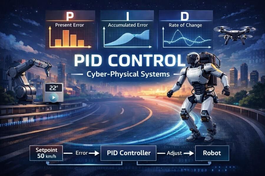
Welcome to the world of PID controllers — the invisible pilots of cyber-physical systems.
A PID controller works in a closed-loop system by continuously measuring the car’s speed and comparing it to the desired setpoint. The difference, called the error, is used to calculate the controller output, which is the control signal sent to the throttle. The actual output (the real, measured speed) is constantly compared to the setpoint, and any disturbances—like hills or wind—affect this actual output, which the controller must correct. This control signal is determined by the combined effects of proportional, integral, and derivative actions, allowing the system to adjust and maintain the target speed despite disturbances. In modern cars, digital controllers implement PID algorithms, providing precise and flexible control through advanced electronic systems.
Historically, James Clerk Maxwell’s 1868 paper ‘On Governors’ laid the theoretical groundwork for control stability, which influenced later developments. The concept of PID control was first formally developed in 1922 by Nicolas Minorsky while researching automatic ship steering for the US Navy.
1. From Software to Physics: The Cyber-Physical Challenge
In software, things are easy.
If you want a variable to be 50, you write:
1 | speed = 50; |
In the physical world, nothing is that obedient.
Cars, robots, drones, heaters, motors — they all live in a messy universe ruled by:
Friction
Inertia
Delays
Noise
Uncertainty
All these factors contribute to complex system dynamics, which affect how the system responds to input signals.
To analyze and predict these responses, engineers use the plant transfer function to model the system’s open-loop response. The transfer function mathematically relates the input signals to the system’s output, allowing for analysis of system behavior and the design of effective controllers.
This is why we talk about Cyber-Physical Systems (CPS):
Cyber → software, algorithms, logic
Physical → motion, temperature, forces, energy
The challenge of CPS is simple to state and hard to solve:
How can software continuously correct the physical world?
To do this, the system must interpret input signals representing deviations from the desired setpoint, and respond accordingly.
The answer is: feedback.
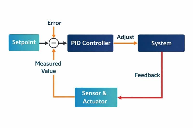
2. The Feedback Loop: Learning by Looking
Let’s go back to our car.
Every few milliseconds, the system does the same thing:
Measure the current speed (the measured process variable)
Compare it to the desired speed (50 km/h)
Compute the error
- The difference between the desired speed (setpoint) and the measured process variable is called the error signal.
- Decide how much to accelerate or decelerate
- The controller uses the error signal to compute the control output, which determines the control action (e.g., how much to accelerate or decelerate).
- Repeat forever
With each cycle, the controller attempts to minimize the error by adjusting the control variable, making ongoing efforts to reach the desired setpoint.
This is a feedback loop.
This entire process forms a control loop, which continuously monitors the process variable and adjusts the system to minimize the error signal.
The system doesn’t assume it is correct. It checks, reacts, and adjusts — constantly.
This simple idea is the backbone of:
Robotics
Autonomous vehicles
Industrial automation
Smart devices
And at the center of this loop sits a small but powerful algorithm: PID.
Types of Controllers
When it comes to teaching machines how to behave, not all controllers are created equal. Just like you wouldn’t use a hammer for every job, control systems use different types of controllers depending on the task at hand.
The most basic is the proportional controller. This controller reacts to the current error between the desired setpoint and the actual measured value. It’s simple, fast, and often used in systems where a quick correction is more important than perfect accuracy—think of basic motion control systems or simple temperature control setups. However, proportional control alone can leave a residual error, known as steady-state error, especially when the system faces constant disturbances. The closed loop transfer function for a proportional controller determines how quickly the system responds and how much steady-state error remains.
To tackle this, engineers often turn to the proportional-integral (PI) controller. In pi control, the combination of proportional and integral actions allows the controller to remember past errors and work to eliminate any persistent offset. This makes PI controllers a popular choice in industrial automation and chemical processes, where maintaining the exact target value over time is crucial. The closed loop transfer function for a PI controller influences system response characteristics such as overshoot and settling time. PI controllers excel at removing offset but can overshoot.
For even more precise and stable control, especially in systems with complex dynamics, the proportional-integral-derivative (PID) controller comes into play. The PID controller combines all three actions—proportional, integral, and derivative—allowing it to react to current errors, correct past mistakes, and anticipate future behavior. The closed loop transfer function for a PID controller is key to balancing speed, accuracy, and stability, affecting overshoot, settling time, and steady-state error. This makes PID control loops the gold standard in everything from industrial robotics to embedded systems, where accurate control and system stability are non-negotiable. The output is divided or distributed over time or across different control scenarios to optimize system performance. PD controllers offer faster response but struggle with steady-state errors and are sensitive to noise.
Of course, there are also specialized controllers designed for unique challenges, such as adaptive controllers or model predictive controllers, but the vast majority of real-world applications rely on the power and simplicity of proportional, proportional-integral, and proportional-integral-derivative controllers.
Choosing the right controller—and tuning its parameters—can make all the difference in achieving optimal control performance, whether you’re keeping a robot arm steady, regulating a control valve, or ensuring your car’s cruise control feels just right. PID controllers are the most comprehensive control solution, balancing speed, accuracy, and stability by combining P, I, and D terms.
3. Meeting PID: Three Simple Questions
A PID controller is not one idea — it is three very human instincts combined. PID controller design involves combining three core controller parameters—proportional, integral, and derivative—to achieve optimal control. These control parameters (proportional, integral, and derivative gains) are tuned to optimize system stability, response time, and disturbance rejection.
Every time the system asks:
How wrong am I right now? → P
Have I been wrong for a long time? → I
Am I getting closer too fast? → D
The PID controller uses these three methods to apply corrective actions by adjusting the controller parameters for optimal performance.
By the way, here is a great video from Digikey that explains really well how a PID controller works:
Let’s explore P, I and D through our story.
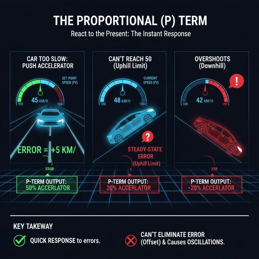
4. P Is for Proportional Control: Reacting to the Present
Imagine you are driving manually.
You look at the speedometer:
45 km/h → you press the accelerator
49 km/h → just a tiny push
60 km/h → you slow down
That instinct is Proportional control.
The bigger the error, the stronger the reaction. The proportional term applies a correction proportional to the current error.
5.1 Formula
The proportional control output is calculated as:
Output = Kp × Error
where Kp is the proportional gain. The proportional gain determines how strongly the controller responds to the current error. A higher Kp increases the response, reducing rise time, but can also cause overshoot or instability if set too high.
5.2 The catch
Proportional control alone cannot eliminate all error. At steady state, a non zero error remains because a non-zero error is required to generate a control output. This means the system will settle with a small, persistent error unless additional control action is used.
Formula (for the curious)
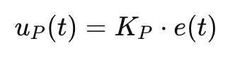
(uP(t)=KP⋅e(t))
Where:
e(t) is the speed error
KP defines how aggressive you are
The Catch
With P alone, the car often stabilizes close to 50 km/h… but not exactly.
Why?
Because physics pushes back.
This small remaining difference is called steady-state error.
To fix that, the system needs memory.
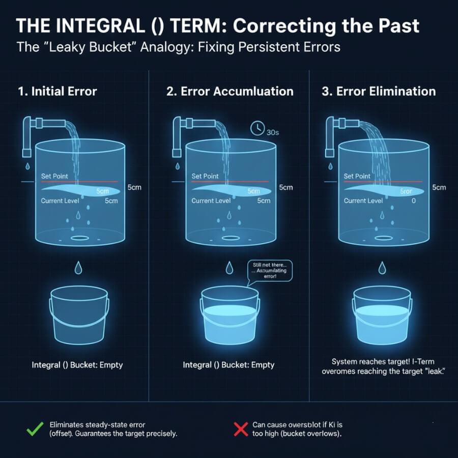
5. I Is for Integral Control: Remembering the Past
Let’s say your car stays at 48 km/h for several seconds.
You don’t just react once — you get annoyed.
“Why are we still slow? Push more.”
That frustration is the Integral term. Integral control accumulates past errors to eliminate steady-state error, ensuring the system doesn’t settle for being close to the target but actually reaches it.
The integral:
Adds up error over time
Punishes long-lasting mistakes
Forces the system to eventually reach the target
**Formula (6.2):**The integral component is mathematically represented as Ki times the sum of past errors, where Ki is the integral gain. Increasing the integral gain accelerates error correction and helps eliminate steady-state offset, but if set too high, it can cause oscillations or instability.
The integral (I) component considers the cumulative sum of past errors to address any residual steady-state errors that persist over time.
No-Math Explanation of an Integral
Think of a stopwatch:
Every second you are wrong → the timer increases
The longer the error lasts → the stronger the correction
Formula
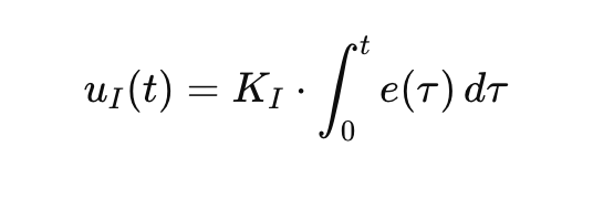
(uI(t)=KI⋅∫0te(τ) dτ)
The Danger
Too much integral turns patience into obsession:
Overshoot
Oscillations
Instability
So we add one last instinct: anticipation.
PI Controller: When Two Are Enough
Not every control system needs the full power of a PID controller. Sometimes, just two ingredients are enough to get the job done. Enter the PI controller—short for Proportional-Integral controller.
A PI controller combines the strengths of proportional control and integral control to deliver accurate control in systems where the dynamics are relatively slow and the requirements aren’t too extreme. Here’s how it works: the proportional part reacts to the current error between the desired setpoint and the actual process variable, providing an immediate correction. Meanwhile, the integral part keeps track of past errors, gradually nudging the control signal to eliminate any lingering offset.
This combination is especially popular in motion control systems, where you might need to control the position or speed of a motor. The proportional integral action ensures that the system responds quickly to changes, while the integral control makes sure that any steady-state error is wiped out over time. The result? A control system that’s both responsive and precise, without the added complexity of derivative action.
PI controllers are a go-to solution in many industrial settings, from regulating flow rates in pipelines to keeping conveyor belts running at the right speed. By focusing on the current error and the accumulation of past errors, a PI controller delivers the kind of accurate control that keeps processes running smoothly—without overcomplicating things.
6. D Is for Derivative Control: Predicting the Future
Imagine accelerating toward 50 km/h very fast.
Even before reaching 50, you already know:
“At this rate, I’m going to overshoot.”
That foresight is Derivative control.
In the PID controller formula, the derivative term is multiplied by the derivative gain (Kd). The derivative gain determines how strongly the controller reacts to the rate of change of the error. Increasing the derivative gain can reduce oscillations and improve system stability by making the controller more responsive to rapid changes.
The derivative (D) component predicts future error by assessing the rate of change of the error, which helps to mitigate overshoot and enhance system stability.
Derivative asks:
How fast is the error changing?
Are we approaching the target too aggressively?
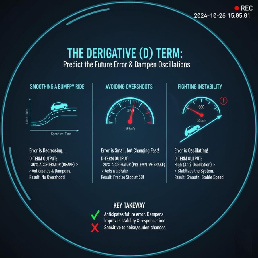
Simple Explanation of a Derivative
A derivative is like sensing momentum:
Fast change → caution
Slow change → relax
Formula
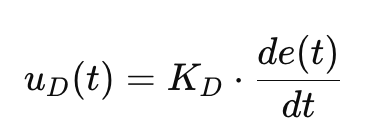
(uD(t)=KD⋅dt/de(t))
Derivative acts like a shock absorber for control systems.
7. The Full PID Controller (At Last)
Put everything together:
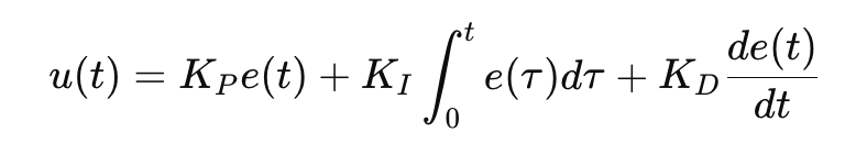
(u(t)=KPe(t)+KI∫0te(τ)dτ+KDdtde(t))
Here, Kp, Ki, and Kd are the PID parameters that determine the strength of each control action—proportional, integral, and derivative, respectively. The combined output of the PID controller, u(t), serves as the control input to the system, adjusting the actuator to minimize the error between the desired and actual values.
Or in human language:
React now (P)Fix what has been wrong for too long (I)Slow down before it’s too late (D)
This combination is surprisingly powerful. The PID controller uses three methods to apply corrective actions: proportional, integral, and derivative.
PID Tuning: Finding the Sweet Spot
A PID controller is only as good as its settings. That’s where PID tuning comes in—the art (and science) of finding the perfect balance between proportional gain, integral gain, and derivative gain to achieve optimal control performance.
Tuning a PID controller means adjusting its parameters so the system responds just right to changes in the input signal. Too aggressive, and you might get wild oscillations; too timid, and the system could be sluggish or never quite reach the target. The goal is to set the PID parameters so the control system reacts quickly, settles smoothly, and maintains stability.
There are several ways to approach PID tuning. Manual tuning is the hands-on method: you tweak the proportional gain, integral gain, and derivative gain while watching how the system responds to a step change in the input signal. It’s a bit of trial and error, but it gives you a feel for how each parameter affects control performance.
For a more systematic approach, engineers often use the Ziegler-Nichols method. This technique involves pushing the system to the edge of stability and measuring its open loop response—specifically, the oscillation period and amplitude. From there, you apply a set of rules to calculate the optimal PID parameters.
Another popular method is the Cohen-Coon method, which uses the system’s open loop response to a step input to derive equations for setting the proportional, integral, and derivative gains. This approach is especially useful for processes with slow dynamics or significant delays.
No matter which method you choose, careful PID tuning is essential for achieving optimal control and getting the most out of your control system.
8. Why PID Is Everywhere in Cyber-Physical Systems
PID controllers are not trendy — they are reliable.
They:
Run in real time
Work on cheap hardware
Are easy to understand
Fail predictably
PID controllers are widely used in various industries, including manufacturing, photonics, and automation, due to their versatility and effectiveness. PID controllers can be implemented without detailed knowledge of the system, making them versatile and cost-effective.
That’s why PID still controls:
Robot joints
Drone altitude
Motor speed
Temperature
Pressure
Vehicle cruise control
Flow rate and level in manufacturing processes such as chemical processing, water treatment, and food production facilities
PID controllers are integral in industrial automation for controlling parameters such as pressure, flow rate, level, and pH within manufacturing processes.
Programmable logic controllers (PLCs) often integrate multiple PID controllers to manage complex industrial processes, providing flexible and programmable control. Digital controllers are widely used in modern systems for their flexibility and performance, allowing multiple PID loops to operate simultaneously in advanced control architectures.
PID controllers are also widely employed in various aspects of everyday life and industrial automation, such as flow controllers in pipes and managing vehicle traffic.
Even modern AI-powered systems often rely on PID at the lowest level to keep physics under control. The integration of PID controllers with modern technologies, such as IoT and artificial intelligence, is shaping their future applications and capabilities.
Applications of PID Control
It’s no exaggeration to say that PID control is everywhere. From the factory floor to the latest industrial robots, PID controllers are the backbone of modern automation and process control.
In industrial processes, PID control is used to regulate everything from temperature and pressure to flow rate and chemical concentration. Whether it’s keeping a reactor at the perfect temperature or ensuring a pump delivers the right amount of fluid, PID control provides the accurate, reliable performance that manufacturing demands.
Industrial robots rely on PID control to move with precision and repeatability. Each joint and actuator in a robot arm is governed by a closed loop control system, using PID algorithms to track the desired position, velocity, or force. This allows robots to perform delicate assembly tasks, weld with accuracy, or handle materials safely.
Temperature control is another classic application. From ovens and furnaces to climate control in buildings, PID controllers keep temperatures steady by constantly adjusting the control output to match the setpoint, compensating for disturbances and changes in the environment.
But the reach of PID control doesn’t stop there. It’s used in everything from automotive cruise control to chemical processing, water treatment, and even in the precise movements of camera gimbals. In many cases, PID control is combined with other strategies—like feedforward or advanced feedback control—to achieve even tighter regulation and better performance.
The reason for PID’s popularity is simple: it delivers accurate control, adapts to a wide range of systems, and is robust enough for the demands of real-world applications. Whether you’re fine-tuning a manufacturing process or programming the next generation of industrial robots, PID control is the trusted tool that keeps everything running smoothly.
9. When PID Reaches Its Limits
PID is not magic.
It struggles when:
Systems are highly nonlinear
Delays are large
Dynamics change constantly
PID controllers are sensitive to changes in system behavior and system dynamics, and may require careful tuning to maintain optimal performance. Understanding system behavior is crucial, as improper tuning can lead to instability or poor response to disturbances.
That’s when engineers add:
Feedforward control
Model Predictive Control (MPC)
State-space methods
Learning-based approaches
But even then, PID often remains the safety net.
10. Final Thought: Why PID Matters
PID controllers teach us a deep lesson:
Intelligence is not about knowing the future.
It’s about correcting mistakes fast enough.
PID is where:
Software meets physics
Theory meets reality
Control becomes intuition
And once you truly understand PID,
cyber-physical systems stop feeling mysterious — and start feeling human.