
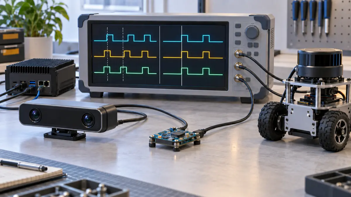
A camera frame arrives ten milliseconds after exposure, yet the perception node reports that it is eighty milliseconds old. The team reduces queue depth, moves inference onto the GPU, and tunes the executor. None of those changes fixes a seventy-millisecond difference between the camera computer’s clock and the consumer’s clock.
The opposite failure is harder to notice: an old observation appears fresh because the publisher’s clock is ahead. An age check can pass while the robot acts on a world that no longer exists.
In ROS 2, a trustworthy timestamp needs an acquisition meaning, an identified clock domain, a conversion into the consumer’s time base, and a bound on conversion error. Use those properties for sensor alignment and freshness. Use a local monotonic clock for elapsed hardware timeouts. After a device restart or time discontinuity, invalidate the affected mapping and dependent state before admitting observations again.
This is a different question from allocating a sensor-to-actuator timing budget. That budget asks how much delay the robot can tolerate. The clock contract establishes whether the delay you calculated is meaningful.
A timestamp says less than its type suggests
The ROS 2 Header definition contains a timestamp and a coordinate-frame identifier. It does not carry a clock identifier, synchronization uncertainty, or device boot identifier. frame_id identifies geometry; it is not a place to encode clock provenance.
Two messages can therefore contain numerically similar timestamps while describing different timelines. Two hosts using system time still need synchronization. Two counters measured in nanoseconds since boot do not acquire a common origin because they use the same unit.
Start by identifying the clocks on the actual robot:
| Clock domain | Useful role | What must be established before comparison |
|---|---|---|
| Sensor or MCU counter | Capture an event close to the hardware | Tick rate, origin, rollover, restart identity, mapping to the robot timeline |
| Host system clock | Shared event timestamps when hosts are synchronized | Time scale, offset/error bound, synchronization health and clock-step policy |
| ROS time | Algorithm time in live operation or simulation/replay | Which source is active and whether all participating nodes use it consistently |
| Local steady clock | Measure elapsed time within one running host | Same clock instance/domain, suitable behavior across suspend, no comparison with another host’s steady clock |
The ROS 2 clock design distinguishes system, steady and ROS time. ROS time follows system time when its override is inactive; a node configured with use_sim_time can instead follow /clock. That timeline may pause or jump backwards. Merely publishing /clock does not synchronize the operating-system clocks or hardware clocks of a robot.
Keep the live sensor timeline and the local timeout timeline separate in your design documents. A hardware lease should expire after real elapsed time even if an estimator’s replay clock has stopped. A steady-clock watchdog still needs reliable execution: an executor that never schedules its callback cannot enforce a deadline. Put the physical fallback on a controller with the required independence, and qualify suspend/resume behavior explicitly.
Record the acquisition event before choosing a clock service
“Camera timestamp” is an incomplete specification. Does it mean exposure start, exposure midpoint, transfer completion, driver dequeue, or publication?
The ROS Image message specifies acquisition time, but the integration still needs to establish the camera driver’s precise convention. A rolling-shutter frame spans time; one header cannot express every row’s exposure. If motion distortion matters, preserve the sensor’s row timing or exposure metadata and use a model that supports it.
A LaserScan has a more specific convention: its header refers to the first ray, and time_increment expresses the interval between measurements. Treating the whole scan as an instantaneous observation can introduce motion error even when every machine’s clock is perfectly aligned.
For AI perception, keep the observation timestamp through inference. A detector that finishes at 14:02:10.200 should not relabel an image captured at 14:02:10.050 as a new observation. Store completion time separately. For a model consuming several frames, preserve the input interval and identify which observation supports the output being used for control.
A useful driver review begins with this contract. These are proposed application fields, not additions already present in standard ROS messages:
| Contract field | Example meaning | Responsible component |
|---|---|---|
| Acquisition event | Exposure midpoint, first laser ray, encoder latch | Sensor integration owner |
| Raw clock identity and units | camera_counter, microseconds | Driver |
| Boot/session identity | Changes when the device restarts | Device or supervising driver |
| Counter rules | Width, rollover handling, discontinuity detection | Driver |
| Conversion record | Scale, offset, reference point, validity interval, mapping version | Time-mapping service |
| Error bound | Maximum qualified conversion and timestamping error under stated conditions | Integration owner |
| Output time domain | Live synchronized system timeline or a named replay session | Launch/runtime owner |
| Failure behavior | Mark timing invalid; prohibit use by the affected motion path | Consumer and supervisor |
Preserve this information in a driver envelope or diagnostic side channel without breaking standard message semantics. The evidence must join unambiguously to a sample: use a source identifier, session identifier and acquisition sequence in your wrapper or trace. A timestamp alone is a poor join key around resets and duplicate samples.
This adds the missing provenance to sensor-fusion drift investigations. Otherwise, “the IMU leads the camera” can mean either a real acquisition difference or a bad conversion.
Turn clock error into an admission calculation
Over a qualified interval, a device counter can often be mapped to the reference timeline using an affine model:
1 | estimated_sample_time = reference_time_at_anchor |
The scale converts ticks and accounts for estimated rate difference. Anchoring the calculation near the data avoids unnecessary numerical precision loss from multiplying large absolute counters. This approximation needs a validity interval and an error bound; it is not a permanent calibration.
Suppose the mapped acquisition time has maximum error u_sample, and the consumer’s reference-clock reading has maximum error u_now. Both errors must be bounded relative to the same timeline. A conservative age interval is:
1 | estimated_age = reference_now - estimated_sample_time |
Adding bounds makes no independence assumption. Combining standard deviations by root-sum-square would require a different statistical argument. A synchronization daemon’s average offset or RMS residual is not automatically a maximum error bound.
Consider a worked example, not a measured robot benchmark. A motion path permits observations up to 40 ms old. A sample appears 28 ms old, but the qualified combined timing uncertainty is 15 ms. Its possible age reaches 43 ms, so that path cannot accept it as satisfying the limit. Looking only at 28 ms would pass an observation whose freshness has not been established.
A conservative admission procedure is:
- Require the expected source session, timeline and valid mapping version.
- Require a current error bound justified for the operating conditions.
- Reject a timestamp definitely in the future:
age_upper < 0indicates a broken assumption or timestamp convention. - Admit for this freshness condition only when
age_upper <= max_age.
If the interval crosses zero, do not silently clamp the estimated age to zero. Record the uncertainty and enforce a separately qualified maximum uncertainty for the consumer. A fresh-but-poorly-timed observation may still be unsuitable for fusion.
That distinction matters. Two observations can each be fresh enough and still be badly aligned with each other. For acquisition times mapped into one domain, a conservative pairwise separation bound is:
1 | maximum_pair_separation = abs(mapped_time_A - mapped_time_B) + u_A + u_B |
Use the actual acquisition conventions in that calculation. An exposure midpoint and the start of a long scan are not interchangeable events.
These bounds can feed a sensor-confidence gate, but keep “clock mapping invalid” distinct from “message arrived late.” They require different repairs.
Synchronizing hosts does not synchronize every sensor
A practical time graph might be:
1 | site reference -> Ethernet hardware clock -> host system clock |
Every arrow needs evidence. Installing a time daemon on the Jetson establishes neither the camera arrow nor the MCU arrow.
LinuxPTP’s phc2sys documentation describes synchronization between a PTP hardware clock and the system clock. It also explains the PTP/UTC time-scale relationship. Check the whole path: a synchronized network-interface clock does not prove that the clock used by the publisher is synchronized, and a time-scale mistake can produce a large fixed offset.
Choose NTP, PTP, hardware triggering or a device-specific conversion against the required error bound and supported hardware. Avoid a universal “PTP means microsecond accuracy” assumption. Validate the deployed interfaces, timestamp location, network path and sensor behavior. A common trigger can align acquisition events, but it still needs a defined relationship to the timestamps attached to them.
For a free-running MCU, packet arrival times alone mix oscillator offset with transport and scheduling delay. A round-trip exchange can help estimate the mapping, but asymmetric delays remain an error source. Preserve that uncertainty instead of fitting a reassuring straight line through biased measurements.
Loss of synchronization is also a time-varying condition. As an illustrative holdover model, a qualified relative frequency-error bound of 20 parts per million contributes up to 1.2 ms of additional timing uncertainty over 60 seconds. Add initial offset uncertainty and other errors. Do not reuse that number without characterizing the actual oscillators, temperature range and mapping method.
The operations signal should therefore include last trustworthy synchronization time, current mapping version, uncertainty growth and restart state. A green process-health indicator for the daemon is insufficient.
Message filters cannot repair a clock-domain mistake
ROS 2 message_filters associates messages using their header timestamps. Exact and approximate matching policies decide which supplied timestamps can form a group. They do not measure the physical offset between two sensor oscillators.
Increasing the matching tolerance can make callbacks resume while making fusion worse. The correct order is to validate acquisition semantics and clock conversion, then choose a pairing tolerance consistent with the estimator’s motion model.
Likewise, replacing a hardware acquisition stamp with now() can conceal transfer delay. It changes the question from “when was the world observed?” to “when did this software stage see the message?” Keep receive time as a separate diagnostic measurement.
Use two measurements while debugging: sample age in a validated common timeline, and processing duration measured locally with a steady clock. If processing duration rises under GPU load while clock error stays bounded, investigate compute or queuing. If age becomes negative while local processing stays stable, investigate the timestamp source and mapping. Neither observation alone proves the root cause, but the distinction prevents blind executor tuning.
Treat resets and replay as changes of timeline
A camera reconnects and its counter returns to zero. An MCU wraps a finite-width timer. A host clock steps during startup. A bag loops to its first message. All four events can invalidate assumptions, but they should not receive the same handling.
A known counter rollover can preserve continuity if the driver unwraps it correctly and no ambiguous sampling gap occurred. A device reboot requires a new session identity and a new mapping. A replay seek requires invalidating temporal state tied to the previous playback position.
Use an explicit recovery transition for affected consumers:
1 | TIMING_VALID |
This is an application pattern, not a built-in ROS 2 state machine. Suspend acceptance before clearing synchronizer queues, estimator history or affected transform caches. Coordinate the transition so an in-flight callback cannot repopulate them with old-session data. Review the reset behavior of each library; do not assume every cache follows a clock jump automatically.
The affected motion path needs its own degraded-mode response. Some robots can continue using independently qualified sensors; others must perform their defined stop or hold behavior. Reinitializing a clock mapping is not, by itself, permission to resume motion.
For replay, align the nodes’ time configuration and keep the replay graph isolated from live actuator endpoints. ROSbag2’s Jazzy documentation distinguishes simulation-time recording from ordinary recording: with --use-sim-time, record timestamps use received /clock values, and recording waits for the first clock message. Those bag timestamps do not replace acquisition stamps inside sensor messages. Preserve both meanings when analyzing a recording.
If replayed algorithms use paused ROS time, a physical hardware watchdog must continue measuring local elapsed time. A test that passes only because both the producer and its timeout froze has not demonstrated a working physical fallback.
Prove the contract with timing faults
Start in an isolated replay environment or a secured test fixture. The point is to perturb time deliberately while preserving enough evidence to distinguish clock failure from sensor failure.
| Injected condition | What the test should establish |
|---|---|
| Constant offset in one source | Age and pairwise alignment checks respond to the qualified bound, even when topic rates stay normal |
| Slow clock drift | Mapping uncertainty grows or is re-estimated; admission changes before the allowed error is exceeded |
| Lost synchronization | Holdover is bounded, observable and eventually expires if qualification cannot be maintained |
| Device restart or counter rollover | A restart cannot reuse an old mapping; qualified rollover handling preserves continuity |
| Replay pause, backward seek and loop | Temporal state resets as designed; local physical timeouts remain effective |
| Delayed inference with fresh publication time | The consumer still evaluates the age of the original observation |
| Apparently future-dated sample | The consumer exposes the timing fault rather than treating negative age as fresh data |
Add a record of the raw acquisition counter, source session, mapping version, mapped stamp, error bound, local receive time and admission result to the robot debug bundle. Preserve mapping history across the fault; the final healthy mapping cannot explain an earlier bad decision.
Before changing a latency threshold, pick one admitted observation and reconstruct its age interval from that evidence. If the team cannot do it, the next task belongs in timestamp provenance and clock qualification. Faster inference will not make an undefined time difference trustworthy.