Encoder Velocity Estimation: Why Low-Speed Robots Jitter

In short: Fix sparse encoder speed feedback with checked count-window calculations, period measurement, explicit stop and reversal handling, and a bench test plan.

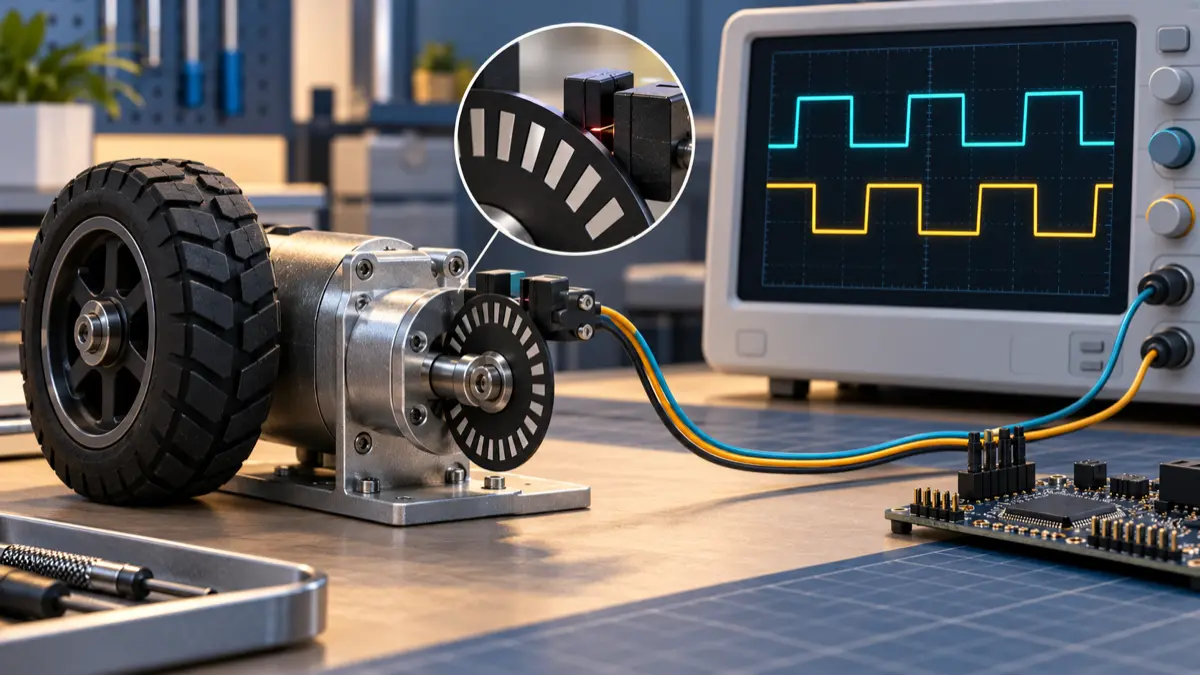
A robot creeps toward its docking station. The velocity loop runs at 1 kHz, but its encoder produces only about 130 counts per second. Most iterations report zero speed. An iteration that sees one count reports more than seven times the intended speed. The controller can end up reacting to the measurement staircase as well as the actual wheel motion.

Before retuning the PID, check how velocity is estimated. Count differences over a fixed window work well when that window contains enough counts. Timing the interval between encoder edges is often more useful at low speed, provided the estimate carries its age and becomes invalid on timeout, capture faults, or direction changes. Neither method turns a sparse position sensor into a continuously observed velocity sensor.

This article develops that choice for a wheel drive, with a reproducible numerical example. The calculations and Python experiment are synthetic; they are not measurements from a robot or a validated motor controller.

Establish what one count means

Use a single unambiguous quantity: decoded counts per wheel revolution, called N below. Record the encoder location, quadrature decoding mode, and transmission ratio next to it.

If a datasheet specifies 512 electrical cycles per encoder-shaft revolution, x4 decoding produces 2,048 transitions per shaft revolution. If that shaft turns 20 times per wheel revolution, the wheel has 40,960 decoded counts per revolution. If the datasheet already specifies decoded counts, multiplying by four again introduces a fourfold scaling error. The abbreviations PPR and CPR are insufficient without the manufacturer’s definition.

Software libraries can normalize the counter too. The WPILib Encoder API explicitly says its distance-per-pulse setting should exclude the decoding multiplier because the library compensates for it. That is a library convention, not a universal formula for a hardware quadrature register.

For the worked example, assume:

• Wheel radius r = 0.050 m.
• Effective resolution N = 2048 decoded counts per wheel revolution, including any gearing.
• Desired constant wheel-rim speed v = 0.020 m/s.
• A velocity-control iteration every 1 ms.

The nominal travel per count is:

q = 2 × pi × r / N
  = 0.000153398 m/count
  = 0.153398 mm/count

count rate = v / q = 130.380 counts/s
edge interval = q / v = 7.6699 ms

Those are wheel-rim quantities under the assumed effective radius. A motor-mounted encoder measures motor motion: gearbox backlash, tire deformation and wheel slip can break the relationship to chassis motion. Keep that distinction when feeding an odometry estimator or an AI planner with a claim about the robot’s actual movement.

Faster differentiation can make the feedback coarser

Let c(t) be the signed decoded count and W the measurement window. The count-window estimate is:

v_count = q × [c(t) - c(t - W)] / W
velocity step = q / W

This is an average over the window. Its output comes in increments of one count divided by the window duration. A faster control loop does not add encoder information; differentiating on every shorter iteration increases that increment.

For the illustrative constant 20 mm/s motion:

Window	Expected counts	One-count speed step	Possible estimates
1 ms	0.130	153.398 mm/s	0 or 153.398 mm/s
10 ms	1.304	15.340 mm/s	15.340 or 30.680 mm/s
50 ms	6.519	3.068 mm/s	18.408 or 21.476 mm/s

A long observation interval makes the average accurate while individual short-window readings remain coarse. With uniform, error-free counts, the difference between measured and true displacement over a window is less than one count; the corresponding speed error is bounded by q/W. This is a quantization bound, not a bound on missed edges, clock error or mechanical error.

There is a useful design test here. Requiring the one-count speed step to be at most 1 mm/s gives:

W >= q / 0.001 = 153.4 ms

A trailing rectangular average of that length represents the motion approximately 76.7 ms in the past for smoothly varying speed. It is not a sensible default for a fast velocity loop. A separate 1 kHz execution schedule does not remove that measurement delay.

This is where PID versus MPC selection meets sensor design: neither controller gets fresh, fine-resolution feedback merely because its computation runs frequently. Choose measurement bandwidth and controller bandwidth together.

Reproduce the staircase before touching hardware

The following standard-library Python program models ideal constant forward motion. It quantizes position into counts and evaluates three non-overlapping windows over ten seconds. It also quantizes ideal edge timestamps to a 1 MHz capture clock.

The assertions check total displacement, the allowed adjacent count levels, and the timer quantization result. There is no motor dynamics model, electrical noise, acceleration, slip or closed-loop controller in this experiment.

from math import floor, pi
from statistics import mean

N = 2048
radius_m = 0.050
speed_mps = 0.020
q = 2 * pi * radius_m / N
phase_counts = 0.37

def count_at(t):
    return floor(phase_counts + speed_mps * t / q)

for window_ms in (1, 10, 50):
    window = window_ms / 1000
    samples = round(10.0 / window)
    deltas = [
        count_at((i + 1) * window) - count_at(i * window)
        for i in range(samples)
    ]
    speeds = [q * dc / window for dc in deltas]
    expected = speed_mps * window / q
    assert set(deltas) <= {floor(expected), floor(expected) + 1}
    assert sum(deltas) == count_at(samples * window) - count_at(0)
    assert abs(mean(speeds) - speed_mps) <= q / (samples * window)
    levels = sorted({round(v * 1000, 3) for v in speeds})
    print(window_ms, "ms:", levels, "mm/s; mean", round(mean(speeds)*1000, 3))

capture_hz = 1_000_000
period_s = q / speed_mps
# Two ideal consecutive edges, both quantized to the same capture clock.
ticks = [round(t * capture_hz) for t in (0.001234, 0.001234 + period_s)]
measured_period = (ticks[1] - ticks[0]) / capture_hz
period_speed = q / measured_period
assert abs(measured_period - period_s) <= 1 / capture_hz
print("period:", round(period_speed * 1000, 3), "mm/s")

The checked output levels match the table; the mean rounds to 20.003 mm/s for all three windows, and the period estimate rounds to 20.000 mm/s. The small mean offset comes from the finite observation interval and quantized endpoints.

Change N, speed and window length to expose the measurement regime of your own design. Do not use the period result as an accuracy claim for an actual encoder: this model gives every count identical angular spacing and perfect edge detection.

Measure elapsed time when counts are sparse

For monotonic motion, measure the elapsed time between accepted capture events separated by m decoded counts:

v_period = direction × m × q / (t_latest - t_previous)

A capture event might occur on every decoded transition, or once per selected group of transitions. Use the actual event spacing in the numerator. Do not combine a once-per-cycle capture interval with a one-transition distance.

Texas Instruments’ eQEP position/speed example illustrates the distinction between counting over a fixed interval for higher speeds and capture-period measurement for lower speeds. Its particular example averages over 64 edges and selects a capture prescaler to avoid overflow. Those settings belong to that example; copying 64 edges into this slow wheel would create an observation interval of roughly 491 ms.

For one-count intervals in our example, a 1 MHz capture clock resolves the 7.6699 ms period into approximately 7,670 ticks. If interval quantization is bounded by one tick, the first-order relative speed error from that quantization alone is about 1/7670, or 0.013%. This is why period measurement can be useful where a 1 ms count difference is mostly zero.

At higher speed, the period contains fewer timer ticks and the same quantization becomes a larger fraction of the interval. Conversely, fixed windows collect more counts. A practical implementation can select between the two methods with hysteresis, using count density and valid capture status rather than a single universal RPM threshold.

Do not overlook edge spacing. A/B phase and duty-cycle errors can make successive x4 transition intervals unequal even at constant shaft speed. Timing equivalent edges a full electrical cycle apart can reduce that particular pattern, at the cost of four-count observation intervals. More averaging buys smoothness by using older information. It does not eliminate physical eccentricity or all encoder error.

A period estimate is already historical

Each estimate describes travel between two past events. Under approximately constant acceleration, associate the interval-average velocity with the midpoint of that interval. At the newest edge in our example, the one-count estimate is already centered about 3.835 ms in the past. Between edges, its age continues to increase.

Publish or retain the measurement interval, the latest edge time, and validity alongside the value. A newly transmitted ROS message containing an old period estimate is not a newly observed wheel speed. The ROS 2 clock-domain guide covers how to preserve that distinction across a microcontroller and host.

Define stops and reversals as estimator states

The most dangerous bug in a reciprocal-period implementation is retaining its last plausible value forever after edges stop. A wheel that was moving at 20 mm/s can keep reporting 20 mm/s while stationary, disconnected, or mechanically blocked.

Choose a maximum acceptable age from the control requirement, then check whether the sensor can support the minimum intended speed. With a 50 ms no-edge timeout and one-count events, the characteristic threshold is:

q / timeout = 0.153398 mm / 0.050 s = 3.068 mm/s

Constant motion slower than this produces edge intervals longer than the timeout. The design cannot both treat every 50 ms silence as stopped and continuously measure arbitrarily slow motion with this sensor. Raising the timeout delays stop/fault recognition; adding resolution changes the trade-off.

Silence is not proof of zero velocity. It could mean slow motion within a count interval, a broken cable, or a stalled mechanism. Expose NO_RECENT_EDGE or another explicit validity state. A controller may apply a separately qualified zero-speed assumption in a known operating mode, but it should not silently treat missing feedback as a precise zero and increase drive effort.

Use the following transition rules as an implementation contract:

Event	Estimator response
Startup or counter reset	Invalidate history; wait for a complete usable interval
Valid same-direction interval	Update value, interval and last-edge timestamp
Direction reversal	Discard the interval spanning the reversal; rebuild from consecutive edges in the new direction
No edge before age limit	Expire the period result; report missing recent feedback
Capture overflow or invalid A/B transition	Invalidate the affected estimate and retain a diagnostic
Counter wrap during normal motion	Apply a bounded modular delta; reject ambiguous deltas

A reversal deserves special treatment because the first reverse edge may cross the same physical boundary that produced the last forward edge. The elapsed time between those two events does not represent one count of net travel. Applying the new sign to the old period is equally wrong. Also, zero net count over a fixed window can hide back-and-forth motion.

For a b-bit position counter, modular subtraction only resolves signed movement unambiguously when the true count change between reads stays strictly within half the counter range. A hardware reset is a different event and needs a new estimator epoch, not wrap correction. Snapshot the counter, capture registers and associated flags consistently so an interrupt cannot pair one interval with another interval’s direction.

Keep edge timing near the motor

Use a quadrature decoder and hardware capture path where the selected device supports them. Timestamping arrival in a Linux or ROS callback includes interrupt, scheduling and transport variation. It measures software service time rather than the physical edge time.

The Microchip dsPIC33A QEI description provides a concrete example of separate position/velocity counters, an interval timer for slow pulses, and configurable input filtering. Check the actual peripheral manual: counter widths, read/reset behavior, capture event selection, overflow flags and filter delays differ across devices.

Qualify input filtering against both noise rejection and the shortest legitimate pulse at maximum speed. A filter that cleans up a stationary bench trace can suppress real transitions at high speed. A clean average speed plot does not prove that counts are preserved.

Keep the velocity loop and estimator together at the actuator boundary, consistent with the microcontroller-versus-Jetson control split. Send the host position, velocity, interval age, method, validity and fault counters. The AI layer can diagnose the recorded evidence or request bounded motion; it should not repair invalid encoder feedback by inventing a smoother speed.

A tracking observer is another option when the count/period trade-off is insufficient. Microchip’s MCAF tracking-loop documentation describes estimating velocity from quantized position and the filtering/phase-lag implications. Its documented near-zero operating limitations also matter: it is a reference for estimator structure, not proof that that implementation supports docking creep. Any observer needs its own bandwidth, reversal and fault qualification.

Qualify the measurement before closing the loop

Begin with a signal generator or a mechanically restrained bench setup appropriate to the drive. Compare captured counts and timestamps with an independent reference. Then evaluate closed-loop behavior under the actual load; static friction, gearbox backlash and current regulation can cause low-speed problems even when the estimator is correct.

Test	Evidence to retain	Acceptance question
Slow constant rotation	Raw count deltas, capture periods, independent speed	Do scale, quantization and age match the predicted regime?
Ramp through method crossover	Both estimates and selected method	Does selection chatter or introduce a control disturbance?
Stop between edges	Last edge, expiry time, validity, drive response	Does the stale result expire within the qualified delay?
Reverse near a count boundary	A/B trace, direction, validity transitions	Is the turnaround interval discarded?
Inject a missing/noisy edge or disconnect	Error flags, count continuity, controller response	Can invalid feedback silently increase drive effort?
Exercise wrap, reset and longest interval	Counter/capture flags and estimator epoch	Are valid wraps distinguished from resets and overflow?

Connect this evidence to the existing sensor-fusion drift investigation only after the wheel measurement itself is understood. Fusion can conceal a bad velocity channel for a while; it does not fix its scale or validity semantics.

For a robot that jitters during creep, the first useful calculation is often counts per control iteration. If the answer is much less than one, inspect the estimator before spending another afternoon on gains. A usable speed signal needs a defined spatial increment, a defined observation interval, and a clear answer when the sensor no longer supports the number being reported.